From JVP to VJP (Part II): By Example
By on 29 May 2025TL;DR
A walk-through of JAX's implementation of autodiff with concrete examples, showing how to derive a Vector-Jacobian Product (VJP) from a Jacobian-Vector Product (JVP).Automatic differentiation is the backbone of all of machine learning and how we build simulation systems at Pasteur Labs. Naively implemented autodiff frameworks usually either suffer from performance inefficiencies or are very hard to implement and maintain for a given programming language. Modern autodiff frameworks like JAX make use of an unholy amount of tricks and abstractions to enable both fast and general gradient computations. The goal of this series of posts is to gain hands-on intuition for how JAX implements autodiff.
This article is a follow-up to From JVP to VJP (Part I), where we explored JAX's approach to automatic differentiation. In Part I, we introduced the concepts of forward mode autodiff via the Jacobian-Vector Product (JVP) and reverse mode autodiff via the Vector-Jacobian Product (VJP). We also mentioned, without going into detail, how JAX uses function overloading and meta-programming to implement autodiff. We learned that JAX derives the Vector-Jacobian Product (VJP) from the Jacobian-Vector Product (JVP), which simplifies the implementation of autodiff (only the JVP needs to know how autodiff actually works) and reduces the number of hand-implemented rules necessary to construct gradients.
In Part II, we will walk through the practical implementation of obtaining a VJP from a JVP in JAX by:
- Computing the JVP and generating an expression of its computation graph
- Separating primal and tangent computation using the linearize operation
- Applying the transpose operation to derive the VJP from the JVP
JAX uses interpreters (or tracers1) to implement function overloading, allowing different types of values to flow through the computation graph.
You can think of JAX's interpreters as a generalization of Python's dunder methods (like __add__).
Examples of interpreters include:
The JVP interpreter, which lets dual numbers flow through the original computation graph.
The
Jaxprinterpreter, which constructs an expression of a function.The
vmapfunction is an interpreter that pushes information along which axis to vectorize through the computation graph.
By stacking interpreters we can express complex transformations in a very concise way.
For example, computing a Jacobian can be expressed as a vmaped JVP (see the takeaways from the previous post).
The Autodidax2 page describes the implementation details of these interpreters. This post will guide you through the interpreters and transformations that happen behind the scenes when you call jax.grad.
The first interpreter we examine constructs a Jaxpr. A Jaxpr is a Python object that represents a computation graph. For example, we can construct the Jaxpr of a function f:
from jax import make_jaxpr
import jax.numpy as jnp

def f(x,y):
  return jnp.sin(x) - jnp.exp(x+y)

make_jaxpr(f)(1., 2.)

> { lambda ; a:f32[] b:f32[]. let
      c:f32[] = sin a
      d:f32[] = add a b
      e:f32[] = exp d
      f:f32[] = sub c e
    in (f,) }
In this example, the Jaxpr represents a function (lambda) with two input parameters a and b of type f32[] (32-bit floating-point scalar), and one output value (f,).
In between we have a list of all the operations that are performed in f in SSA (static single assignment) form. SSA restructures an expression tree into a list of function calls. Each function accepts a number of inputs and has a single, unique output.
SSA is a widely used concept from compiler programming, but is also very useful for autodiff, because it lets you look up the differentiation rules of each function call line-by-line.
To derive VJPs we first need an expression of the JVP. The JVP itself is computed with another interpreter (the JVP interpreter) that
lets dual numbers flow through the original computation graph (as already discussed in Part I).
Interpreters can be stacked, so we can use the Jaxpr interpreter to construct an expression of the JVP computation graph:
from jax import jvp

def df(primals, tangents):
  return jvp(f, primals, tangents)

primals = (1.0, 2.0)
tangents = (1.0, 0.0)

df(primals, tangents)
> (-19.244066, -19.545235)

make_jaxpr(df)(primals, tangents)
> { lambda ; a:f32[] b:f32[] c:f32[] d:f32[]. let
      e:f32[] = sin a
      f:f32[] = cos a
      g:f32[] = mul c f   # a_ * cos a
      h:f32[] = add a b   # a + b
      i:f32[] = add c d   # a_ + b_
      j:f32[] = exp h     # exp(a+b)
      k:f32[] = mul i j   # (a_+b_) * exp(a+b)
      l:f32[] = sub e j   # sin(a) - exp(a+b)                <- primal output
      m:f32[] = sub g k   # (a_ * cos a) - (a_+b_)*exp(a+b)  <- tangent output
   in (l, m) }
We now have a function with 4 inputs (two primals a and b, plus two tangent values c and d), as well as two outputs (one primal and one tangent).
To separate primal from tangent computations, we can rearrange the function calls based on their dependencies on tangent variables (c and d).
Let's annotate each operation of the Jaxpr above that depends on tangent variables with #t-characters:
{ lambda ; a:f32[] b:f32[] c:f32[] d:f32[]. let
    e:f32[] = sin a
    f:f32[] = cos a
    g:f32[] = mul c f   #t: a_ * cos a
    h:f32[] = add a b   # : a + b
    i:f32[] = add c d   #t: a_ + b_
    j:f32[] = exp h     # : exp(a+b)
    k:f32[] = mul i j   #t: (a_+b_) * exp(a+b)
    l:f32[] = sub e j   # : sin(a) - exp(a+b)
    m:f32[] = sub g k   #t: (a_ * cos a) - (a_+b_)*exp(a+b)
  in (l, m) }
By definition of the JVP, all primal computations are independent of tangent computations. This allows us to reorganize the operations, grouping all primal computations at the top:
{ lambda ; a:f32[] b:f32[] c:f32[] d:f32[]. let
    e:f32[] = sin a
    f:f32[] = cos a
    h:f32[] = add a b   # : a + b
    j:f32[] = exp h     # : exp(a+b)
    l:f32[] = sub e j   # : sin(a) - exp(a+b)
  # tangent computations from here on
    g:f32[] = mul c f   #t: a_ * cos a
    i:f32[] = add c d   #t: a_ + b_
    k:f32[] = mul i j   #t: (a_+b_) * exp(a+b)
    m:f32[] = sub g k   #t: (a_ * cos a) - (a_+b_)*exp(a+b)
  in (l, m) }
Note that variables f and j are needed in the tangent computations, even though they are not tangent variables themselves.
They are intermediate results computed during the primal forward pass that we need to make available for the tangent computation.
This is accomplished by keeping track of the variables f and j in an environment (see Eq. 1).
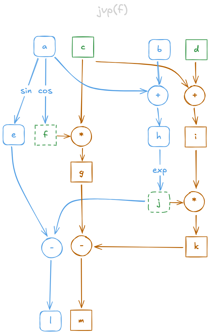
Fig. 1: JVP of the function . Nodes are values, labelled according to the SSA in the code snippet above.
Nodes of the primal computation graph have round corners, nodes of the tangent graph have sharp corners.
Inputs to the tangent are marked in green.
Dashed nodes f and j are computed during the primal and are part of the environment (see Eq. 1).
Linearize / Unzip
The transformation above is called linearize or unzip. We can express it as a function that takes an expression and returns two new expressions: One for the primal computation and one for the tangent computation :
In addition, we get an environment which keeps track of all the variables that were computed during the primal and are needed for the tangent.
You can think of as a dictionary, a cache2, or the variables that closes over. In our example, contains the variables f and j.
In practice, the transformation described above is performed by another interpreter: the partial evaluation interpreter.
JAX constructs a specialized type that marks primals as known and tangents as unknown. This distinction allows to programmatically determine which operations to evaluate immediately (primals) and which to defer to the later JVP computation (tangents).
JAX provides the linearize transformation which extracts the tangent computation into a separate function. This function closes over the necessary primal computation results (specifically variables f and j in our example). To connect with our previous observation, you can think of replacing a -> f and b -> j in the code below to match our manual separation above.
from jax import linearize

primals = (1.0, 2.0)
y, f_jvp = linearize(f, *primals)

tangents = (1.0, 0.0)
f_jvp(*tangents)
> -19.545235

make_jaxpr(f_jvp)(*tangents)
# anything before ';' is the closed over environment E
> { lambda a:f32[] b:f32[]; c:f32[] d:f32[]. let
      e:f32[] = mul c a   # a_ * cos a
      f:f32[] = add c d   # a_ + b_
      g:f32[] = mul f b   # (a_+b_) * exp(a+b)
      h:f32[] = sub e g   # (a_ * cos a) - (a_+b_)*exp(a+b)
    in (h,) }
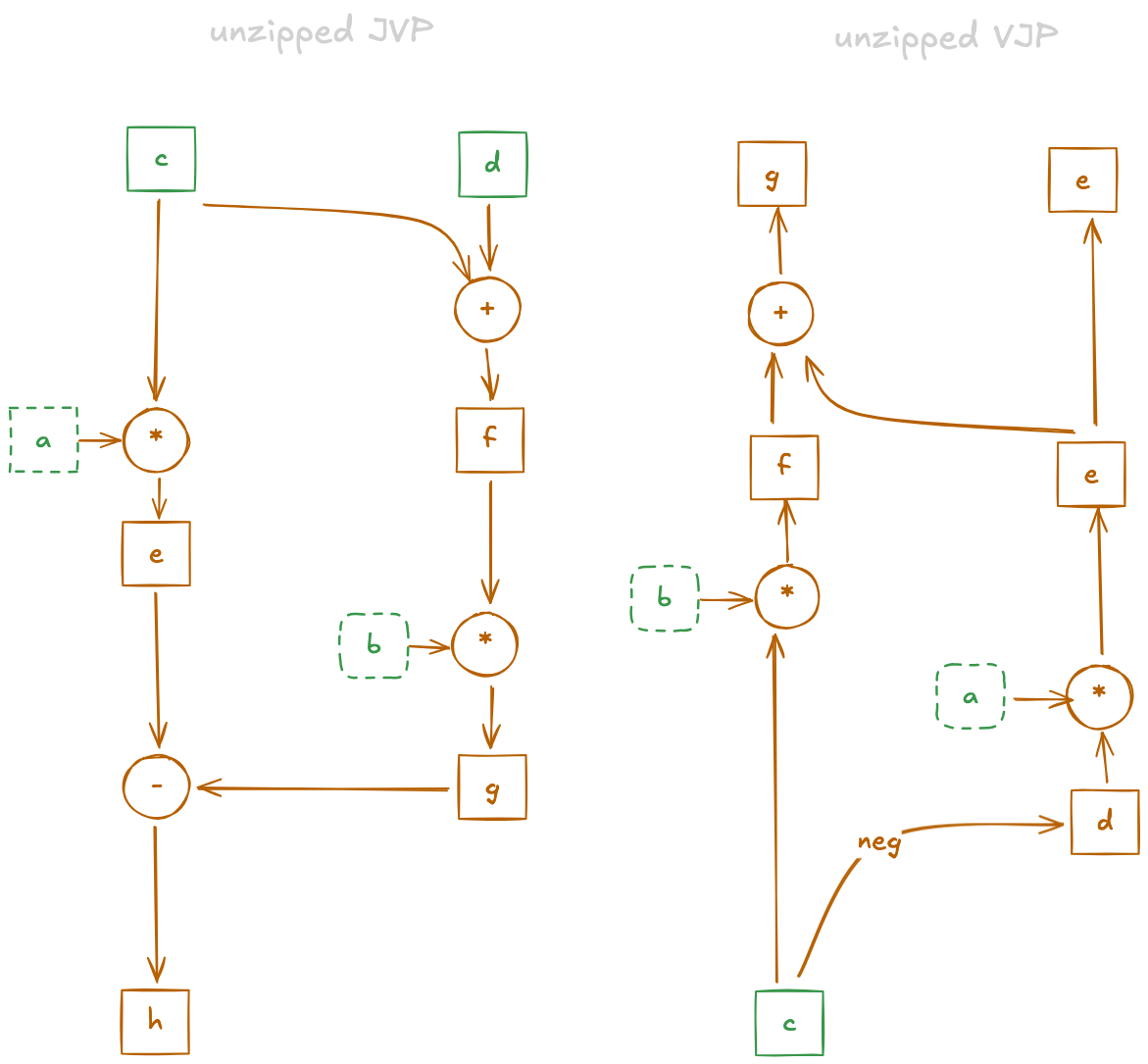
Fig. 2: Comparison of the JVP (left) and VJP (right) of the function . Nodes are values, labelled according to SSA in the corresponding code snippets above.
Inputs to the tangent computations are marked in green.
Dashed nodes a and b (formerly f and j) are computed during the primal and are part of the environment .
Transpose
The transpose transformation effectively reverses the flow of computation of the JVP, which results in a VJP.
Conceptually, this transformation is similar to inverting a function (transforming it from outputs back to inputs, see Fig. 2).
This is done by iterating over the Jaxpr of the tangent computation and applying the transpose rule of each primitive operation in the expression.
Each operation that can end up in the linear, tangent expressions requires its own transpose rule. These rules are applied one by one to transform each operation in the expression. For example, here's how the transpose rule for addition works:
def add_transpose_rule(cotangents, x, y):
  z_bar, = cotangents
  return [z_bar, z_bar]
transpose_rules[add_p] = add_transpose_rule

transpose_rules = {
  "add": add_transpose_rule,
  "mul": ...,
}
Note that the set of transpose rules is much smaller than the set of JVP rules, which simplifies the implementation of the framework. Additionally, it frees JAX users from having to implement both forward and reverse rules when they want custom rules for their own functions (in most cases).
The process of manipulating Jaxprs themselves is called meta-programming.
For those eager to dive into meta-programming with JAX - a good starting point is the inverse_jaxpr function of the tutorial Writing custom interpreters in JAX.
An example of constructing the transpose of a Jaxpr is shown in the function eval_jaxpr_transposed of Autodidax: Part 4.
Applying JAX's linear_transpose transformation to our linearized function yields the VJP function. Unlike the JVP function, which accepts tangents and produces a cotangent output, the VJP function accepts a single cotangent input and produces tangents for each of the original function's inputs.
from jax import linear_transpose

primals = (1.0, 2.0)
f_transp = linear_transpose(f_jvp, *primals)

cotangent = 1.0
f_transp(cotangent)
> (-19.545235, -20.085537)

make_jaxpr(f_transp)(cotangent)
# again, note the closed over environment E with variables a and b
# which were called f and j in the first JVP expression.
> { lambda a:f32[] b:f32[]; c:f32[]. let
      d:f32[] = neg c
      e:f32[] = mul d a
      f:f32[] = mul c b
      g:f32[] = add e f
    in (g, e) }
This final transformation completes our derivation of the VJP. The resulting function f_transp is the VJP of our original function f:
def vjp(f, *primals):
    y, f_jvp = linearize(f, *primals)
    f_vjp = linear_transpose(f_jvp, *primals)
    return y, f_vjp

def grad(f, *primals):
    def grad_fn(*primals):
        y, f_vjp = vjp(f, *primals)
        return f_vjp(np.ones_like(y))
    return grad_fn
Takeaways
We walked through the most important interpreters and transformations that JAX uses for the two different flavors of autodiff: JVP (forward mode) and VJP (reverse mode).
JVPs are computed with a custom interpreter that lets dual numbers flow through the original computation graph.
The
linearizetransformation separates primal and tangent values (of the dual numbers from the JVP) with another interpreter.We applied
linear_transposeto obtain the VJP from the JVP, which reverses the flow of computation and applies the transpose rules for each primitive operation in the tangentJaxpr.JAX's approach to autodiff enables stacking of interpreters, allowing powerful transformations of computation graphs ith minimal and clear code.
Enabling computation on devices other than the CPU (like GPUs/TPUs) becomes straightforward by implementing another interpreter.
Checkpointing can be implemented by clearing the environment and re-computing the necessary variables later.
Footnotes
-
In most of JAX's core code, interpreters are referred to as tracers. But to stay as close to Autodidax2 as we can, we use the word interpreters in this post. ↩
-
If the environment is implemented such that we can clear already computed variables, and re-compute them later, we have effectively implemented checkpointing. ↩