To keep this post brief, we assume familiarity with JAX and automatic differentiation. We also assume some familiarity with forward/reverse autodiff modes.

The team at Pasteur Labs makes heavy use of JAX, an array computing library that employs concepts from functional programming to compile to different hardware, transform programs, and enable automatic differentiation ('autodiff'). Autodiff is a technique to compute gradients of arbitrary programs, forming the backbone of all of machine learning, and how we build simulation systems at Pasteur Labs.

JAX's higher-order primitives (think jax.vmap / jax.jvp / jax.jit) are not just powerful, but also implemented in a new and remarkably beautiful way. This article aims to: (1) summarize how JAX works without the functional programming jargon needed to understand the theoretical paper that underlies JAX, and (2) provide an intuitive insight into JAX's internals.

In the following two sections we will state the absolute minimum you need to know about forward and reverse mode autodiff to understand the third section which describes the novel approach that JAX takes to autodiff. Finally, we provide a few takeaways before concluding this first of several blog posts on autodiff.

Intro: Forward & Reverse Modes

Given a function $f$ and an input $x$, we can implement forward mode autodiff (aka JVP — Jacobian-Vector Product) using dual numbers. To do so we replace $x$ with its dual representation $x + \epsilon v$. Dual numbers have the property that $\epsilon^2 = 0$, which allows us to compute the derivatives of $f$ at $x$ by Taylor-expanding $f(x + \epsilon v)$:

We can use the above approximation to define a dual number as a tuple $(x, v)$. An operation then takes the tuple $(x, v)$ and returns a tuple $(f(x), \partial f(x) v)$:

where the part of the computation related to the "normal" evaluation of $f(x)$ is called the primal, and $\partial f(x)v$ is called the tangent. So, to implement forward autodiff, we have to propagate a tuple of (primal, tangent) through the function $f$. Then we just look up how to propagate a tuple through a given function in a dictionary of jvp_rules:

# instead of
y = exp(sin(x))

# we look up what to do in a ruleset
jvp_rules = {
    "sin": lambda x, dx: (jnp.sin(x), dx*jnp.cos(x)),
    "exp": lambda x, dx: (jnp.exp(x), dx*jnp.exp(x)),
    "add": lambda (x,y), (dx,dy): ((x+y), (dx + dy)),
    "mul": lambda (x,y), (dx,dy): ((x*y), (dx*y + x*dy)),
    # ...
}

a, da = jvp_rules["sin"](/assets/jax/x, 1)
y, dy = jvp_rules["exp"](/assets/jax/a, da)
# dy holds the gradient of exp(sin(x))!

If we devise a way of overloading every numerical function like exp, such that it calls a jvp_rule["exp"] when we want to compute a JVP, we are done! (JAX uses so called Tracers for this — more on implementation details of tracers in Part II.) Most importantly, forward autodiff has only a constant memory overhead compared to the original function. Unfortunately, it requires $N$ evaluations for functions with $N$ inputs, making it prohibitively slow for many machine learning applications.

Reverse mode autodiff (aka VJP — Vector-Jacobian Product) is a bit more tricky.

It propagates derivative information starting from the output to the input. While this enables computing gradients of functions with many inputs and a single output (like most ML loss functions) in one go, its memory complexity grows with the number of numerical operations that are performed in $f$. This is because reverse involves first evaluating the primal (i.e. run $f$), caching all intermediate inputs and vjp_rules, and then composing those rules in reverse (while passing in the correct remembered values, ooof!).

Part I: From JVP to VJP in Pictures

Usually — meaning in all common autodiff frameworks except JAX — forward and reverse mode autodiff require two completely separate implementations. Reverse mode involves much more complicated logic than merely propagating dual numbers forward; it first needs to collect all rules, then reverse them, and finally call them with cached values from the primal. This means implementing compositions of reverse and forward autodiff (which is really what we want when computing things like a hessian) is cumbersome, to say the least.

We can represent any numerical computation as a directed acyclic graph (DAG) with numerical operations as arrows and inputs/outputs as nodes. We will call this the computation graph. In Fig. 1 (left) you can see the computation graph of a simple numerical expression.

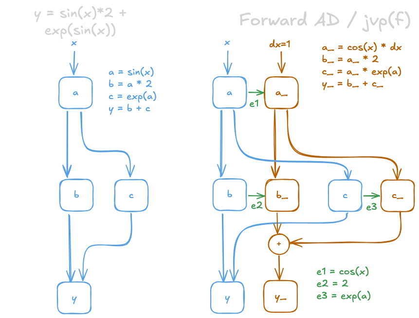
In Fig. 1 (right), we constructed a computation graph corresponding to forward autodiff. It results from pushing a pair of numbers (primal, tangent) through the original graph according to the jvp_rules. The tangent computations are listed in the yellow text box. The green arrows represent values that are required for the tangent computation. However, these values depend on the primal (this becomes important in the next step).

One of the most interesting contributions of the JAX library is acknowledging (and exploiting) that the reverse autodiff computation graph (VJP) looks very similar to the forward autodiff graph (JVP). Essentially, we just have to reverse the yellow arrows, and replace + -> ⌥ / ⌥ -> +. You can verify yourself that the two derivative expressions below are equivalent up to associativity (Fig. 2).

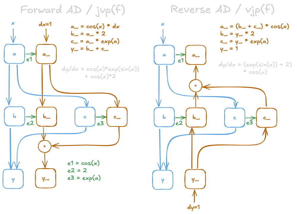
If only we could strip out the yellow part of the computation (left — JVP) we could apply a reasonably straightforward transform to obtain the VJP as sketched below... This is exactly what JAX does! It unzips the primal and tangent computation by partially evaluating the JVP. Partial evaluation means stepping through the primal computation and in the meantime constructing an expression for the tangent, which can be evaluated later. This is where JAX starts using meta-programming techniques — meaning programs that operate on code itself. We will discuss the mechanics of this in Part II of this blog post, but for now you can think of this as follows: The jax.linearize function gives you the value of the primal and a function for the tangent that accepts the green arrows as inputs.

Fig. 3 (left) represents the function returned by jax.linearize. With the green arrows as inputs to this graph all operations within the tangent become linear w.r.t. the inputs, so

hold. This is also what gives jax.linearize its name. The linearity of the tangent means we can invert the tangent graph of the JVP to obtain the VJP! The JVP of $f$ can be reconstructed from Fig. 3:

which is the same as the VJP:

where $a = sin(x)$ as memorized from the forward pass.

The inversion of the linear tangent graph is called transpose, because mathematically, this operation is the transpose of the Jacobian that underlies the gradient of our function. The transpose operation is another case of JAX employing meta-programming as it rewrites the code of the JVP to the VJP.

Interestingly, transposition does not require any information about autodiff. It just needs to know how to invert the yellow arrows. This information is stored in another dict of transpose_rules, which is much smaller than the jvp_rules, because it only has to handle linear operations. This also means that JAX can derive VJP rules from a JVP rule in many cases — cutting the amout of work you have to do for custom rules in half!

Takeaways

JAX implements higher order transformations of computation graphs in two ways:

Function overloading let's us push different values through computation graphs. For example, we can replace single numbers with duals (for the jvp). Or we can replace single numbers with arrays (you guessed it — that is what vmap does)! Function overloading is easily composable:

def jacfwd(f, x):
    pushfwd = lambda v: jvp(f, (x,), (v,))[1]
    vecs_in = np.eye(np.size(x)).reshape(np.shape(x) * 2)
    return vmap(pushfwd, (0,))(vecs_in)

Meta-programming enables manipulation of computation graphs:

def vjp(f, x):
    # delay tangent computations and construct function for linear jvp
    y, f_jvp = jax.linearize(f, x)
    # rewrite jvp to vjp
    f_vjp = lambda y_bar: jax.linear_transpose(f_jvp)(y_bar)
    return y, f_vjp

Both function overloading and meta-programming transformations are composable, so we can do things like:

• Compute reverse mode Jacobian with jacrev(f) = vmap(vjp(f)[1])

• Combine forward and reverse mode to get (a very efficient way of computing) the Hessian: hessian(f) = jacfwd(jacrev(f))

For more details and a thorough proof on how and why linearize and transpose work, we refer to You Only Linearize Once.

Coming soon... from JVP to VJP (Part II): In Practice, where we'll share in-depth examples and explanations of JAX implementation.