Playing Catch With Newton: a Beginner's Guide to Tesseracts
By on 03 Aug 2025TL;DR
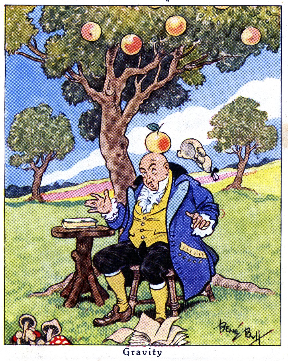
Getting started with Tesseracts? Great! This beginner's guide has you covered with everything you need to build up your basic intuition for how they work. During this tutorial, we demonstrate how you can containerize your physics code for easy distribution, and implement derivative endpoints that can be used in differentiable pipelines.Cover image credit: Isaac Newton discovers gravity, 1936 by René Bull (Meisterdrucke)
Introduction
At Pasteur Labs, we're always looking for ways to speed up scientific progress. We have an ethos: "Don't simplify solutions to scale. Automate complexity to accelerate." Tesseract Core, our latest open source release, embodies this principle — smoothing out the frustrating rough edges between computational tools. No more wrestling with installations, weird interfaces, or duct-taped scripts. Just one consistent way to plug things together. Researchers and engineers regularly make use of fantastic software tools, like physics simulators, machine learning models, meshers, and more. However, these often involve fiddly installation and configuration setups that can be a barrier to adoption for new users.
So how is Tesseract Core any different (and the open-source ecosystem we're building around it), let alone special? It's now possible for researchers and engineers to share working setups of these tools by wrapping them in a "Tesseract", which may be installed for local use with a single command, or even accessed remotely. Better still, all Tesseracts have the same simple JSON interface, which makes switching between Tesseracts or building them into a pipeline a breeze — some call Tesseract Core "Kubernetes for scientific workloads".
But how does this work in practice?
This is the start of a 3-part blog series, acting as a beginner's guide to the Tesseract ecosystem. During these posts, we'll cover how you can:
- Write a Tesseract of your own to share a computational tool
- Use gradient-based techniques to optimise a differentiable Tesseract
- Add interactive web-based user-interfaces to Tesseract optimisations to share your exploratory tools and insights
Who should read this?
This tutorial assumes little existing knowledge of topics such as the Tesseract ecosystem, automatic differentiation, computer aided design (CAD), and the simulation intelligence technologies that are our bread-and-butter at Pasteur Labs. Rather than exploring advanced usage, or focusing on a practical-but-complex use-case, we strip things down to something we can all understand: throwing a ball.
However, some general mathematical and programming knowledge is assumed:
- Basic understanding of differential calculus
- Familiarity with the Python programming language, including it's array-based ecosystem, eg. NumPy and similar libraries
So if you're curious about making Tesseracts of your own, follow along with our basic example. It's fun, and once you're done you'll be equipped to customise it for your own projects.
Physicist's Catch
It's a late summer day in the 17th century, and you are strolling through the Lincolnshire countryside. Quite unexpectedly, you stumble across Isaac Newton beneath his apple tree. He's rubbing his head and staring at a fallen apple when you pass by. To your surprise, when he sees you, he jumps up and challenges you to a game of catch, brandishing his apple with a grin.
As you play, you grow increasingly surprised at his throwing arm. No matter how far you run from him, the apple is propelled into your palm with a perfect trajectory, and you barely have to reach for it! The Natural Philosopher laughs,
"It's just a question of speed and angle! It's easy, there are actually an infinite number of ways I could throw it to you".
Showing off now, he flicks his wrist and the apple whips to you at high speed, with almost no arc (and nearly knocking you on your back), see fig. 1. You toss it back much less impressively and it rolls a few metres wide. Picking it up, he squints upwards, rolls his shoulder, and throws high. The apple soars for a long time, until it is a dot, and then flies back down in a tall arc to your hand, see fig. 2.
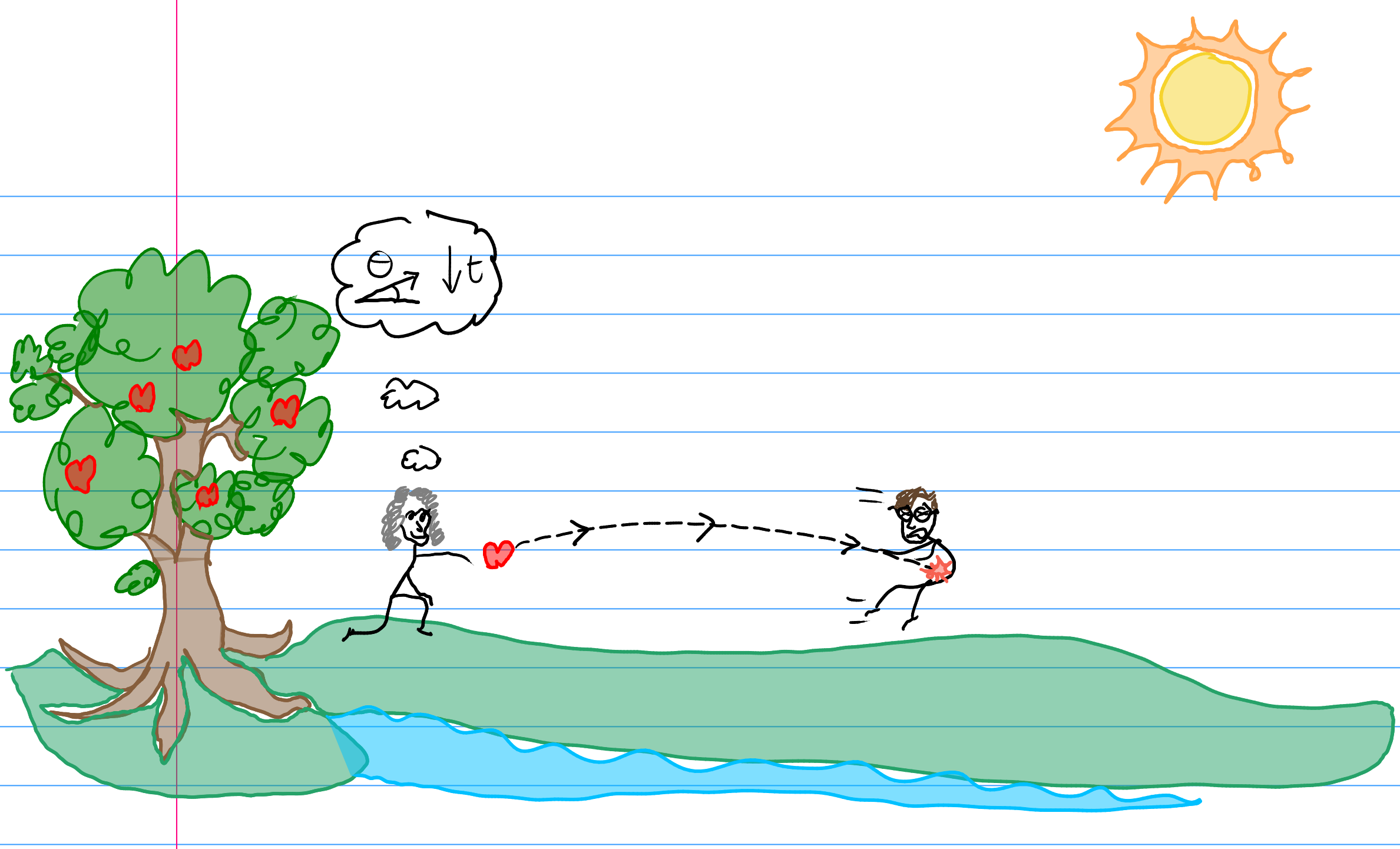
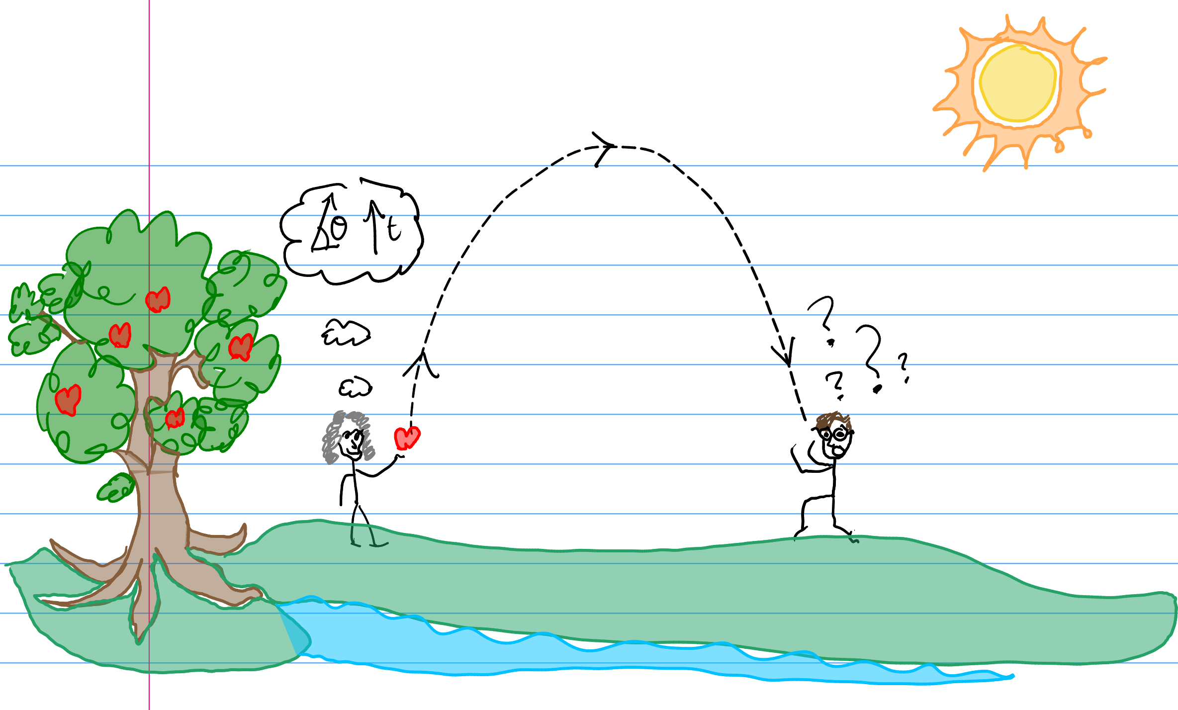
"See?" says Newton, "If you want to give me a real challenge, tell me how long you want the ball to fly before it gets to you. There's only one path for that..."
What was Newton getting at?
Let's throw a ball with maths
Isaac Newton has a lot of relevant stuff to say to us, ranging from the differential calculus which allows us to optimise our algorithms, to the laws of mechanics. Famously, Newton described gravitation via a universal equation (although no apples bonked his head in the process). It's a beautiful and powerful insight, connecting the answers to "why things fall?" and "why do the planets orbit like that?". In fact, his equation is so useful that it forms the bedrock of modern rocket science, centuries after being first written down.
In this post we are, alas, Earth-bound. Unless your throwing arm is really spectacular, you aren't likely to toss a ball high enough to see a difference in its path due to weakening gravity. Instead of using the Law of Gravitation, we opt for Newtonian equations formulated of displacement (), initial velocity (), final velocity (), acceleration (), and time (), respectively (referred to as SUVAT equations by British physicists like me). The simplifying fudge is that is assumed to be constant, and so we can write a simplified equation for the vertical component of a ball's displacement — ie. it's height from the ground — like this:
where is the magnitude of gravitational acceleration (), taken to be 9.81 ms-2.
Recognise it? Well, maybe it's a bit hard to see in maths, but if you plot it, the trajectory looks like this, which should be familiar to anybody who's ever seen a game of catch:

But wait, the equation had height as a function of time; how come this has horizontal distance along the -axis? That's because the horizontal component does not experience any acceleration, so we can just parameterise time as horizontal distance via a simple rescaling:
We find these and components of the velocity by resolving the vector, using basic trigonometry.

So we have
and
Back to Newton's comment about there being only "one path".
Assuming you and Newton are the same height, we can set (things aren't much more complex if we choose another constant) in (3), so that . This means that time is entirely determined by speed and angle. Combining this with (4), we see that as well. So, any pair of coordinates has a one-to-one correspondence with coordinates .
Basically, it all boils down to the following two equations when you combine equations (3) and (4).
Newton had been showing off by using equation (6), plugging in your distance from him, choosing an angle, and then rearranging to get the precise speed he'd need to sling his apple to get to you. He could have chosen any angle he liked (well, except for behind him or into the ground); he'd just need to adjust the speed to toss the apple right to you. Bored, he wants to up the ante by being constrained in and . This instead requires solving (5) and (6) simultaneously, which narrows his options to just one valid speed and angle — only one allowed path.
Putting the maths in a 4D box (defining the problem as a Tesseract)
The maths above is not too complicated. High school physics or maths students could make short work of it. But that's the point: high school physics and maths students can check the back of their books for the answers, and with analytical solutions, so can we!
So, we have a toy physics model with two inputs and two outputs — which we can wrap in a simple Tesseract.
We start by firing up a terminal emulator, creating and entering a fresh directory, then running:
$ tesseract init
which should produce the following files
$ tree
.
├── tesseract_api.py
├── tesseract_config.yaml
└── tesseract_requirements.txt
First some house-keeping. We'll start by giving our Tesseract a name of "projectile" and adding a short description in tesseract_config.yaml, like so:
# Tesseract configuration file
# Generated by tesseract 0.8.1 on 2025-04-04T10:56:02.042524

name: "projectile"
version: "0.0.1"
description: |
    Given a projectile with an initial speed and angle, computes the horizontal
    distance and time-of-flight for it to return to zero vertical displacement.

# ...
Next we can state what dependencies our Tesseract will have.
We are going to use JAX to handle automatic differentiation, so we'll add that to our tesseract_requirements.txt (jax[cuda] if you have access to NVIDIA GPUs).
# Tesseract requirements file
# Generated by tesseract 0.8.1 on 2025-04-04T10:56:02.042524

# Add Python requirements like this:
jax[cuda]==0.5.3

# ...
With that out of the way, we are ready to define our Tesseract itself! We do this by editing tesseract_api.py.
The first thing to do is define our inputs' and outputs' schemas:
from pydantic import BaseModel
from tesseract_core.runtime import Differentiable, Float32


class InputSchema(BaseModel):
    speed: Differentiable[Float32]
    angle: Differentiable[Float32]


class OutputSchema(BaseModel):
    distance: Differentiable[Float32]
    time: Differentiable[Float32]
These are given as Pydantic models (see https://docs.pydantic.dev/latest/concepts/models/) and take the
inputs and outputs you'd expect from equations (5) and (6).
tesseract_core.runtime provides us with some types to extend Pydantic, and here we use Float32.
Since we would like the ability to perform gradient-based optimisation, we wrap this type with the Differentiable[] generic1.
We ultimately want to get a Jacobian, ie. derivatives of the inputs with respect to the outputs,
Rather than doing this by hand, we'll use JAX to perform this derivative2.
First, though, let's write down our functions from (5) and (6) in Python.
import jax
import jax.numpy as jnp

RECIP_GRAV_STRENGTH = 1.0 / 9.81

OUTPUT_FUNCS = {
    "distance": lambda speed, angle: (
        speed * speed * RECIP_GRAV_STRENGTH * jnp.sin(2.0 * angle)
    ),
    "time": lambda speed, angle: (
        2.0 * speed * RECIP_GRAV_STRENGTH * jnp.sin(angle)
    ),
}
Using the JAX function jnp.sin enables JAX to perform autodiff by "tracing" the functions, but that's not a detail we should worry ourselves with.
Just keep in mind that if we use jnp rather than NumPy or the standard math module, it's to make the autodiff work.
To calculate the Jacobian as in (7), we need to differentiate the "distance" function with respect to the "speed" and "angle" parameters, and likewise for the "time" function.
How can we do this with JAX?
JAX exports jax.grad(), which lets you differentiate a function with respect to input parameters.
You just pass the function, along with the numerical index of the input parameter you want to differentiate with respect to, eg. jax.grad(OUTPUT_FUNCS["distance"], argnums=1) is equivalent to .
This is a little unclear; we want to fill out the full Jacobian, so should iterate through all inputs / outputs, and it would be nice to have a mapping by name, eg. accessing GRAD_FUNCS["distance"]["angle"] to retrieve the gradient function for . So let's fill that nested dictionary by looping through the parameter names at the inner level.
We can get them using the inspect module.
import inspect
import typing

def arg_names(func: typing.Callable[[...], typing.Any]) -> list[str]:
    """Returns the names of the arguments of a function, in order."""
    return inspect.getfullargspec(func).args
So that our GRAD_FUNCS dictionary is:
GRAD_FUNCS = {
    output_name: {
        input_name: jax.grad(func, argnums=num)
        for num, input_name in enumerate(arg_names(func))
    }
    for output_name, func in OUTPUT_FUNCS.items()
}
Great! So now we have a dictionary of output functions, and a nested dict of dicts whose inner elements are gradient functions of the outputs.
We expose this to the Tesseract endpoints via the apply() and jacobian() functions. The apply() function is simple, we just call the functions in OUTPUT_FUNCS:
def apply(inputs: InputSchema) -> OutputSchema:
    return OutputSchema(
        distance=OUTPUT_FUNCS["distance"](
            speed=inputs.speed, angle=inputs.angle
        ),
        time=OUTPUT_FUNCS["time"](speed=inputs.speed, angle=inputs.angle),
    )
The jacobian() function needs a tiny bit more massaging.
It should return a dictionary with the exact same structure as GRAD_FUNCS, but with the elements replaced with the floating point output of the corresponding gradient function.
Basically, we just need to loop through the nested structure and evaluate the functions, nothing too major.
from collections import defaultdict
from itertools import product

def jacobian(
    inputs: InputSchema,
    jac_inputs: set[str],
    jac_outputs: set[str]
) -> dict[str, dict[str, float]]:
    grads = defaultdict(dict)  # empty dict instantiated if value missing
    for output_name, input_name in product(jac_outputs, jac_inputs):
        grads[output_name][input_name] = GRAD_FUNCS[output_name][input_name](
            inputs.speed, inputs.angle
        ).item()
    return dict(grads)
If you're wondering what the point of jac_inputs and jac_outputs is, don't worry!
Diligent authors of Tesseracts naturally want to give their users as many options for their optimisations as possible.
However, Tesseract users won't typically need to optimise every output with respect to every input.
So jac_inputs and jac_outputs just gives them the option to only compute what they need for their specific optimisation problem.
And with that, we're done writing our Tesseract! Let's build it and see if it's behaving as expected.
How's your throwing arm? Building and testing your Tesseract!
If you've been following along with the CLI commands, and copypasta'ing code snippets, you should be ready for the next step. If not, feel free to clone the repo here and jump in.
So now we have a Tesseract defined, we jump into our terminal emulator, cd into the right directory and execute the following:
$ tesseract build .
If everything is installed properly on your system, then that should be it — the Tesseract is ready to run! You can do this three ways; via the:
- CLI
- Python API
- REST API
See Interacting with Tesseracts for more info. For the purpose of testing in this post, we will use the CLI, although in the next one we will make use of the Python API for more programmatic control.
We can access the apply() function we coded above, passing it parameters for speed and angle, using the following command:
$ tesseract run projectile apply '{"inputs": {"speed": 10.0, "angle": 0.75}}' | jq .
{
  "distance": {
    "object_type": "array",
    "shape": [],
    "dtype": "float32",
    "data": {
      "buffer": 10.168144226074219,
      "encoding": "json"
    }
  },
  "time": {
    "object_type": "array",
    "shape": [],
    "dtype": "float32",
    "data": {
      "buffer": 1.3896815776824951,
      "encoding": "json"
    }
  }
}
Where we have piped the output to jq to make the JSON formatting a bit prettier.
Using Standard International units, with radians for angles, we can plug this into our equations (5) and (6), and we find this is correct. Admittedly, this is slightly underwhelming, though, since we almost wrote our maths verbatim in code. More excitingly, let's see our Jacobian output!
$ tesseract run projectile jacobian '{"inputs": {"speed": 10.0, "angle": 0.75}, "jac_inputs": ["speed", "angle"], "jac_outputs": ["distance", "time"]}' | jq .
{
  "time": {
    "speed": {
      "object_type": "array",
      "shape": [],
      "dtype": "float64",
      "data": {
        "buffer": 0.13896815478801727,
        "encoding": "json"
      }
    },
    "angle": {
      "object_type": "array",
      "shape": [],
      "dtype": "float64",
      "data": {
        "buffer": 1.49172043800354,
        "encoding": "json"
      }
    }
  },
  "distance": {
    "speed": {
      "object_type": "array",
      "shape": [],
      "dtype": "float64",
      "data": {
        "buffer": 2.0336289405822754,
        "encoding": "json"
      }
    },
    "angle": {
      "object_type": "array",
      "shape": [],
      "dtype": "float64",
      "data": {
        "buffer": 1.442144751548767,
        "encoding": "json"
      }
    }
  }
}
Rewriting (7) with the actual derivatives, and then evaluating:
So just like that, we confirm that we have correctly automatically evaluated the gradients of the distance and time of flight of our ball, with respect to angle and speed. Newton would be proud! Although you'll need to wait for the next post to see how we can optimise our Tesseracts, to finally best him at this game of Physicist's Catch.
Wrapping up
So by writing a simple toy physics model, we have shown that we can represent the input and output interface simply in Python, wrap our model in the same file, and expose the inputs / outputs via the Tesseract's standard apply() and jacobian() endpoints (see Tesseract endpoints for more).
We've shared our source code with you on GitHub, so you can run the Tesseract we wrote today with minimal setup. And now you have all the skills you need to get started with wrapping your own favourite tools in Tesseracts. Go forth and share them — we'd love to see how you put it to use!
You can share your creations and thoughts with us, and our growing community, on the official Tesseract Forum. This is also a great place to have your questions answered by our Tesseract experts and developers!
Tune in for the next post in this series, which covers what you might do if you stumbled across a great Tesseract that you'd like to put to work for your own optimisation tasks. See you soon!
Footnotes
-
See the docs on
Array[]to learn how to go beyond scalar inputs. ↩ -
For improved efficiency and reduced user-required modification, you might consider using the
tesseract init --recipe jaxcommand. This inserts a template with advanced-usage JAX code, automatically defining VJPs and JVPs based on a singleapply_jit()function definition. To keep things transparent here, we will use a more naïve setup. ↩